
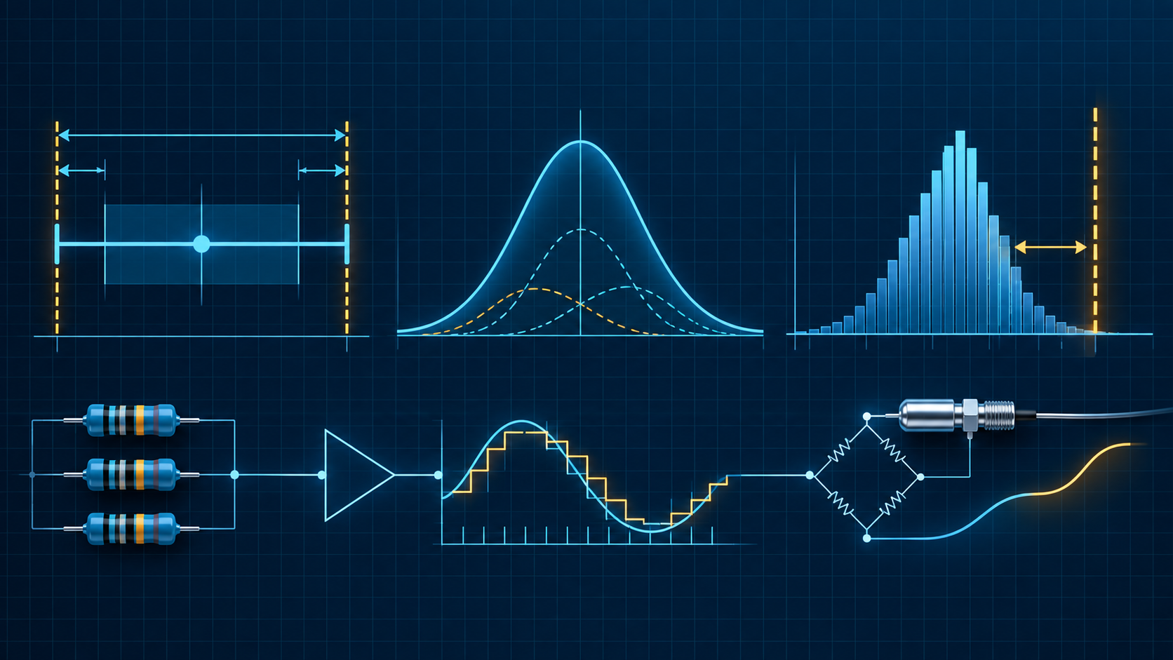
Tolerances and worst-case analysis
Build a reliable error budget: worst-case addition, RSS, Monte Carlo simulation, and design margin for resistors, ADCs, and RTD sensors.
Written and technically reviewed byElectroDesignForge Engineering Team
View the editorial processKey point: worst-case analysis proves that a product stays within its limits for every permitted combination of parameters. RSS estimates typical spread when errors are independent and random. Monte Carlo makes the distribution visible. None of the three replaces margin: margin protects against omitted effects, drift, and ageing.
Quick reference
| Method | Formula for contributions e_i | It answers | Use it when |
|---|---|---|---|
| Worst case | `E_WC = Σ | e_i | ` |
| RSS | E_RSS = √(Σ e_i²) | “What typical spread should I expect?” | independent, centred errors that can be treated as standard deviations |
| Monte Carlo | random draws through the model | “What are the distribution and escape rate?” | nonlinear model, known distributions, or correlations |
| Margin | distance to limit after the budget | “What is left for reality?” | always, before freezing a design |
Every error must be referred to the same output quantity before combination: ADC input volts, ohms, degrees Celsius, gain percentage, or ADC codes. A ±1% tolerance is not automatically a 1% standard deviation.
Start with a measurable requirement
Write the transfer function and limits before choosing a method. For a resistor divider read by an ADC:
V_meas = V_exc × R_low / (R_high + R_low)
0.10 V ≤ V_meas ≤ 3.20 V
For a temperature chain, the requirement may be temperature error ≤ ±0.5 °C from −20 to +80 °C. For an ADC, it may be “never saturate at maximum signal” or “total error below 2 LSB.” Each contribution is then expressed in the unit of that requirement.
Keep these terms distinct:
- tolerance: a stated component or reference limit;
- drift: change with temperature, age, voltage, or time;
- error: deviation of the result from truth;
- uncertainty: interval or spread assigned to an estimate;
- margin: deliberate headroom between the worst-case result and the limit.
Tolerance addition: the worst-case budget
When a contribution can degrade the output by e_i in one direction, add magnitudes:
E_WC = |e_1| + |e_2| + … + |e_n|
This assumes every variable reaches its harmful extreme simultaneously. It is conservative, but appropriate when the specification must be met for every unit, when datasheet limits are guaranteed, or when an output can saturate.
Example: ADC reference and divider
A measurement must remain within ±20 mV. After referring every term to the measured node:
| Maximum contribution | Input-referred error |
|---|---|
Divider ratio (resistors ±0.1%) | ±4 mV |
| ADC reference: initial accuracy | ±5 mV |
| ADC reference: temperature drift | ±3 mV |
| ADC offset | ±2 mV |
| Filtered noise, conservative bound | ±1 mV |
E_WC = 4 + 5 + 3 + 2 + 1 = ±15 mV
margin = 20 − 15 = 5 mV, or 25% of the limit
Do not cancel two bounds without proof: a positive reference error and a harmful divider ratio can coexist. For a multiplicative quantity (gain, R × C), first calculate high and low corners, or use percentage terms for small deviations.
RSS: quadratic addition, not “lighter worst case”
For independent, centred errors already expressed as standard deviations σ_i, the combined standard deviation is:
σ_total = √(σ_1² + σ_2² + … + σ_n²)
A coverage band follows the chosen level: roughly ±1σ covers 68.3% of a normal distribution, ±2σ 95.4%, and ±3σ 99.7%. Therefore, never RSS raw “±x%” tolerances without knowing what they represent.
If a resistor is specified at ±1% as a bounded uniform production limit, a common approximation is σ ≈ 1% / √3. If a datasheet already states a ±3σ limit, then σ = limit / 3. These conversions are assumptions: retain them in the budget and prefer manufacturer distribution data when available.
When RSS becomes wrong
- Contributions are correlated: two resistors in the same network drift together, one reference feeds many channels, or temperature affects several terms.
- A term is a deterministic limit: guaranteed absolute accuracy, calibration bias, software clamp, or supply excursion.
- The result approaches saturation: clipping is nonlinear and asymmetric.
- Tails are unknown or distributions are strongly non-normal.
In those cases, keep the deterministic term outside RSS, or introduce covariance. For two terms, σ² = σ_1² + σ_2² + 2ρσ_1σ_2, where ρ is their correlation. At ρ = 1, statistical benefit vanishes: the contributions add.
Monte Carlo: see the model’s actual distribution
Monte Carlo does not replace the model; it repeats it with randomly drawn inputs. The workflow is straightforward:
- Write the output relationship and compliance limits.
- Assign every input a justified distribution: bounded uniform, normal, measured law, or real production lot.
- Encode correlations: shared ambient temperature or a common lot are not independent draws.
- Run enough trials, then record mean, standard deviation, percentiles, and out-of-limit fraction.
- Repeat with changed assumptions to check that the conclusion is robust.
For example, 100,000 trials can characterize a tail around 10⁻3, but cannot prove a 10⁻6 escape rate. For very-low-defect requirements, combine tail analysis, guaranteed limits, and production validation; do not claim “zero defects” merely because no draw showed one.
Monte Carlo is especially useful for RTD nonlinearity, a linearization polynomial, the exact divider ratio, or volts-to-codes conversion in an ADC. It also reveals a shifted distribution: a narrow spread around a biased mean is still a bad result.
Margin: the reserve that makes a budget usable
For an upper limit L_max and calculated maximum output y_max:
absolute margin = L_max − y_max
relative margin = (L_max − y_max) / L_max × 100%
For a range, calculate margin to each bound and keep the smallest. Margin is not an “extra error” to blindly RSS: it is a design choice that absorbs unmodelled effects, lot variation, assembly, ageing, test conditions, and future changes.
Document the target, for example “at least 20% ADC full-scale headroom” or “at least 0.1 °C after the worst-case budget.” Margin in physical units is often clearer than a percentage close to zero.
Practical case: RTD + ADC chain
Consider a Pt100 with excitation current, lead resistance, amplifier, and ADC. At a chosen temperature, refer each effect to °C:
| Effect | Example treatment |
|---|---|
| IEC 60751 RTD class | sensor limit, generally part of the worst-case budget |
| 2/3/4-wire leads | calculate resistance and mismatch at thermal extremes |
| Self-heating | use maximum current and the real assembly’s thermal coefficient |
| Reference and analogue gain | convert errors to °C through local sensitivity dV/dT |
| ADC offset, INL, and noise | convert V or LSB to °C at the same temperature point |
| Linearization | check algorithm error, resolution, and rounding |
Sensitivity is not constant across the range. The same 1 mV can represent more degrees in one part of the curve than another. Run the budget at several corners: low, mid, and high temperature; supply and ambient extremes; sensor and component limits.
Recommended workflow
- List the requirement, operating range, limits, and output unit.
- Collect every contribution: initial specification, temperature, time, supply, noise, quantization, assembly, and calibration.
- Write each term’s sign and sensitivity; transform it to the output unit.
- Run worst-case corners first. Eliminate every saturation or negative margin.
- Add RSS only for truly statistical and independent terms, with an explicit coverage level.
- Simulate Monte Carlo for nonlinear models, measured distributions, and yield trade-offs.
- Allocate and verify remaining margin at all corners, including after calibration if calibration belongs to the product.
- Validate hardware with a measurement method more accurate than the specification being demonstrated.
Common pitfalls
- Adding percentage tolerances that are not referred to the same output.
- Using RSS on datasheet limits as though they were standard deviations.
- Omitting temperature drift, ageing, reference voltage, or lead resistance.
- Assuming independence when contributions share temperature, lot, supply, or calibration.
- Reading a Monte Carlo result as a worst-case guarantee.
- Reserving margin only at nominal; useful margin is calculated after the budget.
Associated calculators
- Open the Resistor tolerance calculator to combine initial tolerance and TCR over the temperature range.
- Open the ADC/DAC calculator to check LSB, quantization, input range, and conversion codes.
- Open the RTD lab to compare 2/3/4-wire wiring, sensor error, self-heating, and ADC resolution.
Sources
- JCGM 100:2008 — Evaluation of measurement data — Guide to the expression of uncertainty in measurement (GUM).
- NIST Technical Note 1297 — Guidelines for Evaluating and Expressing the Uncertainty of NIST Measurement Results.
- IEC 60751 — industrial platinum resistance sensors and tolerance classes.
- Datasheets for the selected voltage reference, ADC, amplifier, and RTD.